BridgeLoRA

IIntroduction

Large language models (LLMs) are increasingly deployed in privacy-sensitive domains such as medical triage involving patient records, contract analysis of confidential documents, and personal assistants handling private communications. In many tasks, effective deployment benefits from LLM fine-tuning with sensitive data that resides on edge devices which helps preserve privacy, improve inference accuracy, and reduce inference-time prompt length. However, edge devices typically lack the computation capacity to fine-tune billion-parameter models locally, while offloading fine-tuning to the cloud exposes sensitive information, including raw inputs, labels, and training gradients to the cloud. This creates a fundamental challenge in the edge-cloud continuum, i.e., achieving server-grade computation capability without exposing task-specific information during fine-tuning.

There exists a privacy-computation trade-off, i.e., full local training preserves privacy but is often computationally prohibitive, whereas offloading alleviates the burden on edge devices at the cost of potentially revealing raw inputs, labels, trainable parameters, or gradients depending on how computation is partitioned between edge and server. Therefore, a practical edge–server fine-tuning system must satisfy three simultaneous constraints:

1. Exposure Minimization: minimize the sensitive information accessible to the cloud—ideally excluding raw inputs, labels, loss values, and trainable-module parameters/gradients;
2. Lightweight Edge Computation: the edge executes and updates only lightweight modules while the heavy backbone computation is offloaded to the server; and
3. Communication Efficiency: round-trips and transfer volume must not dominate training step time under WAN latency and bandwidth limits.

Existing approaches face fundamental trade-offs: split learning methods like SplitLoRA²⁰ and MobiLLM²¹ partition computation between edge and cloud but expose task-specific parameters or gradients to the server, while skip adapters like Skip2-LoRA⁸ target single-device efficiency rather than distributed privacy.

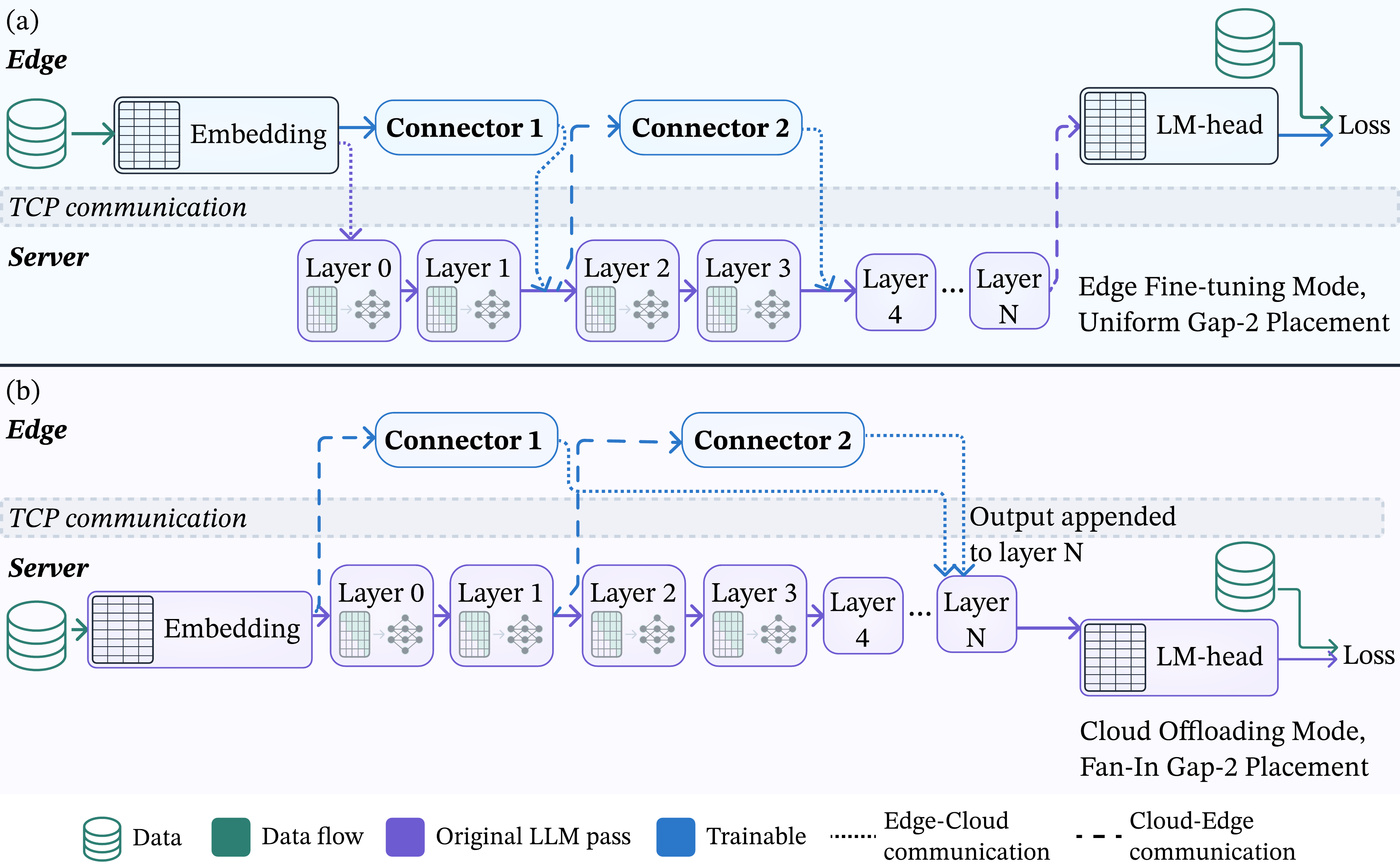
We contribute BridgeLoRA, a fine-tuning framework at the edge leveraging skip connectors^22,8. These are small trainable modules that bridge $d > 1$ frozen transformer layers, reducing synchronization from $O(L)$ to $O(L/d)$ for an $L$-layer model while enabling computation-communication overlap. BridgeLoRA supports two modes, i.e., Edge Fine-tuning Mode and Cloud Offloading Mode. Edge Fine-tuning Mode keeps labels, loss, and trainable parameters at the edge, while Cloud Offloading Mode moves embeddings and loss computation to the cloud server. On the Aya multilingual instruction-tuning dataset²⁹, transformer skip connectors outperform standard LoRA on the same model (1.47 vs. 1.66 validation loss on Llama-3.2-3B) while training 2.7% of parameters, and distributed testbed results show latency mainly affects wall-clock time (44% overhead at 500 ms) with similar model quality. To the best of our knowledge, BridgeLoRA is the first effort to leverage skip connectors for privacy-aware distributed LLM fine-tuning.

Our contributions are threefold:

• Exposure-minimizing edge–server framework: BridgeLoRA uses skip connectors with an explicit threat model that keeps task-specific parameters, their gradients, and (in Edge Fine-tuning Mode) the labels and loss on the edge, while reducing synchronization frequency and overlapping transfers with frozen-backbone computation.
• Connector design space and configuration guidance: A deliberate expressiveness gradient (LoRA, GLU-FFN, Transformer) is evaluated across skip distances 2–30 and two placement strategies on Llama-3.2-3B and Qwen3-4B, with hyperparameter robustness sufficient that we offer a default-recipe cookbook for selecting connector type, gap, and placement under deployment constraints.
• Communication optimizations validated on distributed testbed: Connector placement strategies and gradient compression techniques achieve up to 40× bandwidth reduction with minimal quality loss.

Our framework is released at https://github.com/vimeto/bridge-lora.

IIRelated Work

Parameter-Efficient Fine-Tuning

Modern LLMs are typically fine-tuned using parameter-efficient methods that add small trainable modules while freezing the backbone. Adapters³ insert bottleneck feed-forward modules at each transformer layer, while LoRA¹ attaches low-rank weight updates in parallel to the model's weight matrices, enabling task adaptation by training less than 0.5% of parameters. QLoRA² extends this approach to 4-bit quantized models, enabling fine-tuning of 65B-parameter LLMs on consumer hardware. Other variants include prefix tuning⁴ and prompt tuning⁵, which optimize learnable tokens rather than weights. One challenge is adapter sizing. Marouf et al.⁶ observe that very low-dimensional adapters perform poorly and propose MiMi for learned dimension selection. However, existing methods typically place adapters at every layer, which would require communication at each layer boundary in collaborative settings.

Placement of Adapters and Skip-Connected Adapters

Several works explore sparser adapter placements to balance efficiency and expressiveness. AdapterDrop⁷ removes adapters from lower transformer layers, showing minimal performance loss with approximately 36% inference speedup. Skip-LoRA⁸ adds trainable LoRA adapters between the output of the last layer and the inputs of earlier layers, creating skip connections that bridge multiple layers. This reduces the backward-pass computation by 82–88% relative to LoRA-All. Combined with activation caching in Skip2-LoRA, the authors report up to 90% reduction in fine-tuning time without accuracy loss. However, Skip2-LoRA targets computational efficiency for on-device training rather than privacy-preserving distributed settings.

Dynamic Layer Skipping

LayerDrop⁹ randomly drops layers during training to enable depth reduction in inference, while early-exit networks^10,11 attach intermediate classifiers for early stopping. LayerSkip¹² combines layer dropout with early-exit loss, achieving up to 2.16× speedup. FlexiDepth¹³ adds adapters with learned gates to route tokens through either the full layer or a lightweight path, finding that skipping layers requires learned adapters to prevent representation drift. DiffSkip¹⁴ enables token-wise FFN skipping, showing that a 32-layer LLaMA can skip 8 FFN layers while preserving 91.3% of performance. These techniques demonstrate that learned skip transformations can compensate for bypassed computation, though they focus on single-device efficiency rather than distributed privacy.

Collaborative and Privacy-Preserving Learning

Federated learning¹⁵ trains models across distributed data without centralization, but gradient updates can leak training data¹⁶. Differential privacy¹⁷ mitigates this only at nontrivial accuracy cost. Split learning¹⁸ partitions models between client and server, but Abuadbba et al.¹⁹ demonstrated that intermediate activations at the cut layer are highly correlated with raw input, leading to severe privacy leakage. Recent work combines split learning with parameter-efficient fine-tuning. SplitLoRA²⁰ divides LLMs at a cut layer, with the client handling the early layers and the server handling the later layers and LoRA adapters. MobiLLM²¹ proposes server-assisted side-tuning, training an auxiliary network on the server that is fused with the frozen backbone via summation. However, both approaches expose task-specific parameters or gradients to the server, compromising privacy guarantees. A complementary line uses prompt or prefix tuning^4,5: adapted state takes the form of soft tokens supplied at run time. This fits a server-hosted backbone but is largely orthogonal to our exposure axis, as the server still observes inputs and the adapted state is presented as model input rather than executed within an edge trust boundary. BridgeLoRA instead keeps adapted state as parametric modules on the edge.

Skip Connections in Deep Learning

Residual connections²² enable training of very deep networks through identity shortcuts of the form $x + f(x)$, which facilitate gradient flow and training stability rather than task-specific adaptation. DenseNet²³ and highway networks²⁴ extend this paradigm with learned gating mechanisms, yet these approaches remain fundamentally concerned with within-layer stability rather than cross-layer adaptation. Transformers exhibit layer redundancy²⁵, where not all layers contribute equally to task-specific transformations. This motivates learned skip transformations that can bridge redundant layers, though existing work does not address how such mechanisms could enable privacy-preserving distributed training.

IIIBridgeLoRA

We contribute BridgeLoRA, the first framework to combine skip connectors with distributed edge-server fine-tuning. Although skip connectors⁸ and compression techniques have been studied independently, their combination for privacy-aware collaborative learning represents a novel contribution that enables bridging of multiple layers across a trust boundary while retaining all task-specific parameters at the edge.

Threat model. We assume an honest-but-curious server that executes the protocol but may inspect any data it receives. In Edge Fine-tuning Mode raw inputs, labels, the loss, and all connector parameters/gradients remain on the edge; the server sees only frozen-backbone activations and their gradients. Cloud Offloading Mode relaxes this by moving embeddings and the loss to the server (exposing tokens and labels), while connector parameters and gradients stay on the edge. The exposure-minimization claim is therefore on connector parameters and the gradients of the loss on those parameters, not on the activation-class connector output $\delta_k$. BridgeLoRA provides exposure minimization, not cryptographic privacy: intermediate activations remain a leakage surface via inversion attacks¹⁹.

Skip Connector Architecture

The core architectural innovation of BridgeLoRA pertains to the skip connector. Instead of adapting each layer individually (as in standard LoRA), lightweight modules are trained to bridge multiple frozen layers simultaneously. This reduces the number of synchronization points from $O(L)$ to $O(L/d)$, where $d$ is the skip distance. A skip connector $C_{i \to j}$ maps hidden states from layer $i$ to layer $j$. Importantly, for $j > i+1$, this creates a “skip window” of $d = j-i$ layers:

The skip window $d$ directly controls communication overhead. Consider the protocol for each skip window:

1. Server computes frozen layers $i \to j$, producing $h_j$;
2. Server sends $h_j$ to edge; edge computes connector $C_{i \to j}(h_i)$;
3. Edge sends skip residual $\delta = C_{i \to j}(h_i)$ to server;
4. Server combines: $h'_{j} = h_{j} + \delta$.

With standard per-layer adapters, this exchange occurs $L$ times per forward pass. With skip distance $d$, it occurs only $L/d$ times. For gap-15 on a 28-layer model, synchronization drops from 28 to 2 round-trips—a 93% reduction in cumulative latency overhead. Our distributed experiments (Section V) confirm that latency affects only wall-clock time, not model quality, i.e., at 500ms added latency, training time increases by 44% while validation loss remains unchanged.

We consider two placement strategies. Uniform placement places connectors at regular intervals (e.g., every $d$ layers). This minimizes the maximum distance any signal must travel without correction but incurs $\approx L/d$ synchronization points. Fan-in placement targets all connectors to a single layer (e.g., layer $L-1$), enabling computation-communication overlap, i.e., the server streams intermediate activations to the edge while continuing backbone computation, and the edge computes all connectors in parallel. Synchronization occurs only at the final layer, reducing overhead to $\mathcal{O}(1)$ regardless of connector count.

Design of Connectors

The frozen layers between $i$ and $j$ are not skipped, but continue to run and produce $h_j$. The connector $C_{i \to j}$ instead learns an additive task-specific correction that is added on top of the frozen output (Eq. 1). It must capture the residual that frozen weights cannot, given the bridging distance $d$, the amount of cross-token mixing the correction needs, and how token-dependent it is. We evaluate three architectures (LoRA, GLU-FFN, Transformer) spanning a range of expressivity, each motivated by a distinct hypothesis about which structural property the correction requires.

LoRA Connector

The LoRA connector adapts LoRA¹ to operate in representation space rather than weight space. In contrast to standard LoRA, which modifies layer weights through additive updates ($W + \Delta W$), the skip connector transforms activations across layer boundaries:

where $A \in \mathbb{R}^{H \times r}$ and $B \in \mathbb{R}^{r \times H}$. The matrix $B$ is zero-initialized to preserve pretrained behavior, and the scaling factor $\alpha/r$ controls adaptation magnitude ($\alpha=2r$ by default). This representation-space formulation complements standard weight-space LoRA: skip connectors apply coherent corrections across multiple layers, whereas LoRA performs localized weight modifications within individual layers.

GLU-FFN Connector

The GLU-FFN connector uses a Gated Linear Unit feed-forward network²⁶, computing

where $W_{\text{gate}}, W_{\text{up}} \in \mathbb{R}^{H \times H_{\text{ffn}}}$ and $W_{\text{down}} \in \mathbb{R}^{H_{\text{ffn}} \times H}$. The FFN dimension $H_{\text{ffn}}$ is configurable from 1/8 to full model dimension, enabling parameter-quality trade-offs. All projections are initialized from $\mathcal{N}(0, 0.02^2)$, except $W_{\text{down}}$ which is zero-initialized to ensure identity behavior at training start. The gating mechanism provides non-linear, token-dependent transformations that enable richer adaptations than LoRA's linear projections.

Transformer Connector

The Transformer connector implements a full self-attention block with optional FFN. Let $t = h + \text{Attn}(\text{RMSNorm}(h))$ denote the post-attention state. The connector computes

returning only the delta (final state minus input), so the skip residual can be added by the model. We use configurable attention head count (4–16 heads tested). Q, K, V projections operate on the full hidden dimension. The output projection $O$ and FFN down projection are zero-initialized; all other projections use $\mathcal{N}(0, 0.02^2)$.

Table I summarizes connector parameter counts under gap-2 configuration for Llama-3.2-3B (13 connectors) and Qwen3-4B (17 connectors). LoRA provides extreme efficiency (<0.01% of model parameters), while Transformer connectors maximize expressiveness (2–3%). Head count affects only the attention pattern, not total parameters.

Collaborative Training

Our protocols implement transient synchronous communication, where the edge requires server responses to proceed, but skip connectors reduce the number of synchronization points. We implement two operational modes (Figure 1), trading privacy for efficiency. Algorithm 1 formalizes Edge Fine-tuning Mode; Cloud Offloading Mode is described as a delta from it below.

Training Objective and Trainable Parameters

Both modes share the same training objective and parameter scope; these are design choices of BridgeLoRA, distinct from optimizer and schedule hyperparameters reported in Section IV.

Trainable parameters. We freeze all backbone parameters—embeddings ($W_E$), transformer layers ($\{L_1, \ldots, L_N\}$), and the language model head ($W_{lm}$)—and update only the skip connector parameters $\theta_C$. This reduces trainable parameters from 3–4B to 0.3–200M depending on connector type and count (Table I), and is what enables the lightweight-edge property: the edge holds gradient state and optimizer state only for $\theta_C$.

Loss. The objective is standard next-token prediction,

where gradients flow through the frozen backbone but only $\theta_C$ is updated. In Edge Fine-tuning Mode this loss is computed entirely on the edge from cached labels; in Cloud Offloading Mode the server computes it on labels supplied by the edge.

Edge Fine-tuning Mode (Maximum Privacy)

Algorithm 1 keeps task-specific parameters (connectors, embeddings, LM head) and labels on the edge; server processes only frozen activations. For skip residual $h'_{s_{k+1}} = h_{s_{k+1}} + \delta_k$, gradients flow through both branches: $\nabla h'_{s_k} = \partial \delta_k / \partial h'_{s_k} \cdot \nabla \delta_k + \nabla h_{s_{k+1}}$. Edge caches $h'_{s_k}, \delta_k$ for backpropagation. Server never observes tokens, labels, or connector parameters/gradients.

Cloud Offloading Mode (Maximum Efficiency)

Cloud Offloading Mode is structurally Algorithm 1 with three changes: (i) the embedding $E$ and the LM head $W_{lm}$ move to the server, so the edge sends input_ids/labels and the server now computes the loss; (ii) each skip block runs in parallel—the server sends $h'_{s_k}$ to the edge and computes $h_{s_{k+1}} = L_{s_k+1:s_{k+1}}(h'_{s_k})$ while the edge computes $\delta_k = C_k(h'_{s_k})$, after which the edge returns $\delta_k$ and the server forms $h'_{s_{k+1}} = h_{s_{k+1}} + \delta_k$; and (iii) on the backward pass the edge does not return the connector-input gradient, so the feedthrough term $\partial \delta_k / \partial h'_{s_k}$ is dropped and backbone gradients downstream of $s_k$ propagate only through the residual branch $\nabla h_{s_{k+1}}$. This approximation costs little empirically (Table III) and is what enables the pipelined activation/connector overlap that gives Cloud Mode its speedup.

Bandwidth Optimization (Cross-Mode)

INT8 Quantization². We quantize activations to 8-bit integers before transmission, reducing transfer size by 50% compared to bf16. Our experiments confirm INT8 quantization does not degrade skip connector training quality.

Top-K Gradient Sparsification. We transmit only the top $k\%$ largest-magnitude gradients along with their indices. Our key finding is that skip connector gradients are highly sparse. Top-K at 5% achieves 75% bandwidth reduction with only 0.3% quality degradation (Table IV). Combining INT8 with Top-K 1% achieves 40× compression (97.5% bandwidth reduction) with only 0.9% quality loss, enabling deployment over bandwidth-constrained connections.

IVExperimental Setup

Models

We evaluate Llama-3.2-3B²⁷ (28 layers, $H$=3072, 3B params) and Qwen3-4B²⁸ (36 layers, $H$=2560, 4B params). Both use grouped-query attention, SwiGLU, and rotary embeddings.

Datasets

Our primary dataset is Aya Multilingual SFT²⁹, a curated subset of 9,850 samples balanced across four languages, including Finnish, Swedish, English, and Spanish. We use a 95/5 train/validation split with 9,358 and 492 samples, respectively. Following standard practice in parameter-efficient fine-tuning research^1,2, we use validation loss as the primary metric, as accuracy is uninformative for open-ended generation over large vocabularies without verifiable outputs. Additionally, we evaluate catastrophic forgetting through WikiText-2 perplexity (Section V) and assess cross-domain generalization by additionally training on four diverse datasets:

• FineMath: 10,000 samples of mathematical reasoning and proofs;
• FineWeb2-HQ: 10,000 samples of high-quality general web text;
• OpenThoughts: 10,000 chain-of-thought reasoning traces; and
• Magpie: 10,000 synthetic instruction-following examples.

These span instruction tuning, text continuation, and domain-specific paradigms.

Baselines

We compare against three baselines. Full fine-tuning trains all 3–4B parameters with a lower learning rate of $10^{-5}$ and gradient checkpointing to fit in memory. Standard LoRA¹ applies LoRA adapters on Q, K, V, and O projections at every layer. Sparse LoRA (no skip) (our ablation baseline) places standard LoRA adapters at the same layer positions as skip connectors but without the skip residual connection, testing whether the bridging mechanism is essential or whether sparse adapter placement alone suffices. Throughout the paper, “Skip LoRA” denotes a LoRA connector with the skip residual; the no-residual ablation is always labelled “Sparse LoRA (no skip)” or, in tables, “LoRA at skip positions (no residual)”.

Metrics

Validation Loss: Cross-entropy on held-out Aya data. Primary metric for fine-tuning quality.

WikiText-2 Loss: Perplexity on standard benchmark. Checks for catastrophic forgetting of general language modeling ability.

Connector Count: Number of skip connectors—equivalently, synchronization points per forward pass. Doubles as a coarse exposure-frequency proxy, since each boundary is one activation handoff between edge and server; we treat this as a proxy, not a formal privacy guarantee (Section VI).

Parameter Count: Trainable parameters as percentage of model. Efficiency metric.

Training Details

All experiments use the AdamW optimizer with $\beta_1=0.9$, $\beta_2=0.999$, and weight decay of 0.01. We use learning rates of $10^{-4}$ for LoRA and FFN connectors, $5\times10^{-5}$ for Transformer connectors which benefit from lower rates, and $10^{-5}$ for full fine-tuning. Training uses batch size 4, with 8 GPUs using DDP, and gradient accumulation over 8 steps for an effective batch size of 256, with a cosine learning rate schedule with 10% warmup. Sequence length is 512 tokens for all experiments. We train for 3 epochs (105 optimizer steps) unless noted; extended training results (350+ steps) are indicated where applicable. Mixed precision (bf16) is used for efficiency. Default hyperparameters include LoRA rank 4 with $\alpha=8$, FFN dimension at 1/4 of model hidden size, and Transformer connectors with 8 attention heads.

VExperiments & Evaluation

Skip Connectors vs Baselines

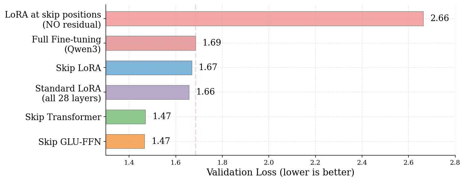
Table II compares skip connector performance against baselines on Llama-3.2-3B. Skip Transformer and GLU-FFN connectors achieve the best results on the validation set (1.47 loss), outperforming standard LoRA (1.66 loss) by 11%. This comparison is not iso-parameter (Transformer: 2.7% vs LoRA: 0.25%); the primary benefits are reduced synchronization frequency and (with fan-in placement) computation-communication overlap, rather than parameter efficiency. Full fine-tuning was run on Qwen3-4B due to resource constraints, achieving comparable results (1.69 loss). The frozen backbone provides implicit regularization that prevents overfitting, as evidenced by the minimal gap between validation loss (Table II) and training loss. Additionally, skip connectors converge in only 3 epochs while full fine-tuning requires longer training, suggesting the skip transformation is inherently simpler to learn than full parameter updates.

Skip LoRA vs. standard LoRA across ranks shows that Skip LoRA consistently outperforms standard LoRA on Llama-3.2-3B while achieving comparable performance on Qwen3-4B, despite using fewer adapters. On Llama-3.2-3B, Skip LoRA outperforms standard LoRA at all ranks despite using fewer adapters (13 vs 28): at rank 16 ($r$=16), Skip LoRA achieves 1.67 loss versus 1.78 for standard LoRA, a 6.2% improvement. On Qwen3-4B, Skip LoRA matches or exceeds standard LoRA performance: at rank 8, Skip LoRA achieves 1.79 versus 1.90 for standard LoRA, despite using only 47% as many adapters (17 vs 36). This suggests that bridging layers provides complementary information flow to per-layer adaptation, and that the skip residual mechanism enables more efficient parameter utilization. This performance difference may also result from adding LoRA adapters only to the attention projections (Q, K, V, and O), rather than the transformer FFN.

LoRA at skip positions without skip residuals achieves only 2.66 loss on Qwen3-4B, which is 0.93 points worse than Skip LoRA with residuals at 1.73 on the same model, demonstrating that the residual bridging mechanism is a key innovation.

Distributed Training Protocols

We validate BridgeLoRA's core claim, that skip connectors enable practical pipelined edge-server communication, using a distributed testbed with actual TCP communication. Our setup uses two nodes on the LUMI supercomputer, each with AMD MI250X GPUs and Slingshot interconnect. The server node runs the frozen backbone across 7 GPUs via DDP; the edge node runs connectors on 1 GPU. Communication uses TCP sockets and PyTorch tensor serialization. Added latency (20–500ms) simulates WAN conditions.

Table III compares Edge Fine-tuning and Cloud Offloading modes on the distributed testbed. Edge-mode wall-clock cost limited Edge runs to ~33 optimizer steps vs. 300–500 for Cloud, so these are protocol-cost comparisons rather than matched-step quality comparisons. At 20 ms, Cloud runs at 56 s/step vs. Edge's 89 s/step (1.6× speedup) because it only transmits connector activations/gradients. Going from 20 ms to 100 ms adds ∼8% in Edge (89→96) and ∼32% in Cloud (56→74); Cloud is more latency-sensitive due to its higher per-step round-trip count.

Bandwidth Optimization

Table IV compares gradient compression methods by validation loss, bandwidth reduction, and compression ratio. The actual bandwidth reduction depends on the serialization format. Each retained gradient requires an 8-byte index plus a 2-byte value, making Top-K at 10% equivalent to INT8 (both 50% reduction). However, Top-K at 5% achieves 75% reduction, and Top-K at 1% achieves 95% reduction. Top-K 5% offers the best single-method trade-off with 75% bandwidth reduction and only 0.3% quality degradation (1.798 vs 1.793 baseline).

The combination of INT8 quantization with Top-K 1% sparsification achieves 40× compression (97.5% bandwidth reduction) with only 0.9% quality degradation (1.810 vs 1.793). For bandwidth-constrained edge deployments over cellular or satellite links, this combined approach makes collaborative fine-tuning practical where it would otherwise be infeasible. Notably, the combined method (1.810) outperforms INT8 alone (1.826) while using 20× less bandwidth, suggesting that aggressive sparsification provides implicit regularization.

Latency Tolerance

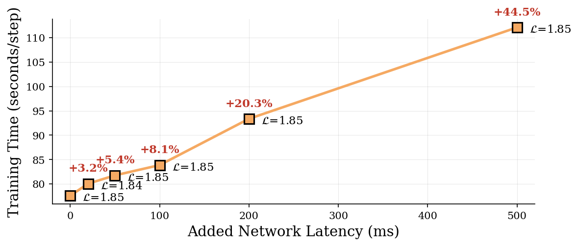
We conduct a systematic latency sweep from 0ms to 500ms added network latency using identical configurations (INT8 + Top-K 1% compression, gap-15). Figure 3 presents the results, with each data point annotated with both the validation loss ($\mathcal{L}$) and the percentage time overhead. The key finding is that added network latency affects only training time, not model quality. Validation loss remains constant at $\mathcal{L}\approx 1.85$ across all latency levels, while training time scales linearly from 77.6 s/step (baseline) to 112.1 s/step at 500ms (+44.5% overhead). This predictable behavior is acceptable for many deployment scenarios and validates that the reduced synchronization frequency from skip connectors (gap-15 reduces round-trips by 85%) enables practical deployment over a wide range of network latencies.

Fan-in Placement

Table V quantifies communication overhead, showing that fan-in placement reduces bandwidth by 7× compared to uniform placement for the same number of connectors by batching all transfers into a single synchronization event. This directly addresses the latency constraint in Cloud Offloading Mode training.

Table VI compares the quality between fan-in and uniform placement. Fan-in placement incurs a quality penalty of 0.35–0.53 loss depending on connector type, with more expressive connectors (Transformer, GLU-FFN) showing smaller degradation than LoRA. The Transformer connector maintains competitive quality at 1.94 loss even with fan-in placement—only 0.25 worse than full fine-tuning (1.69). This trade-off may be acceptable for bandwidth-constrained deployments where the 7× bandwidth reduction outweighs the quality degradation. For applications where communication is the primary bottleneck (e.g., satellite links, cellular networks), fan-in placement with Transformer connectors provides a compelling configuration.

Skip Distance & Connector Count

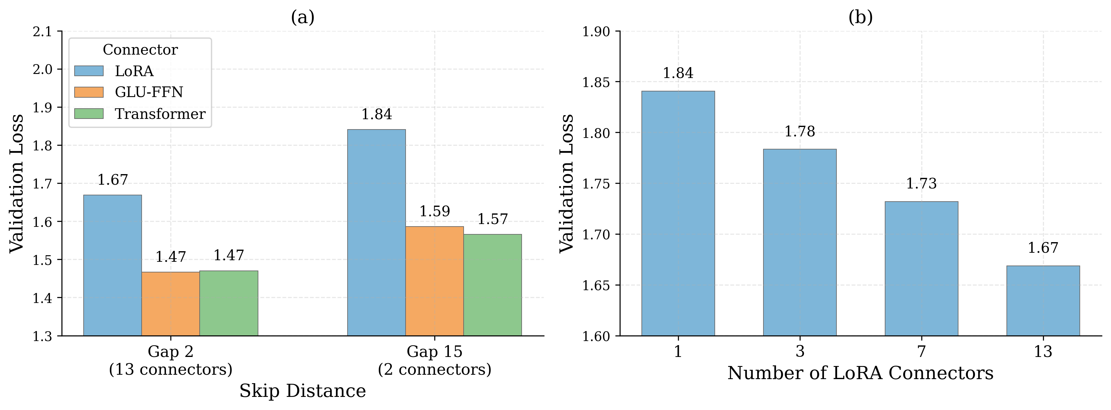
Figure 4(a) and Table VII quantify the quality degradation as skip distance increases. On Llama, increasing skip distance from gap-2 to gap-15 incurs only 0.10–0.12 loss degradation for Transformer and GLU-FFN connectors (1.47→1.57 and 1.47→1.59), while LoRA exhibits larger degradation at 0.17 (1.67→1.84). Since gap-15 reduces connectors from 13 to 2—an 85% reduction in network round-trips—this trade-off may be acceptable for latency-sensitive deployments.

On Qwen3-4B, degradation is somewhat larger due to the deeper architecture (36 vs 28 layers): gap-15 incurs 0.06 loss for Transformer (1.59→1.65), 0.09 for GLU-FFN (1.60→1.69), and 0.08 for LoRA (1.84→1.92). The relative ordering Transformer > GLU-FFN > LoRA remains stable across all skip distances, indicating that the expressiveness advantage of more complex connectors persists as bridging difficulty increases.

We extend to gap-30 on Qwen3-4B with a single connector. Even in this extreme configuration, Transformer connectors achieve 1.82 loss—only 0.23 worse than gap-2, and still competitive with standard LoRA baselines. GLU-FFN achieves 1.88 loss, and LoRA achieves 2.15 loss. The gap-30 results reveal a non-uniform degradation of approximately 0.06–0.17 loss per 13–15 additional layers bridged (smaller from gap-2→15, larger from gap-15→30), reducing network round-trips by 94% compared to gap-2 placement.

Figure 4(b) shows how validation loss scales with connector count. Increasing from 2 to 13 connectors on Llama improves loss 1.84→1.67, and from 3 to 17 connectors on Qwen3 improves 1.96→1.73 (0.23 vs. 0.11 reduction), which is consistent with Qwen3's deeper architecture benefiting more from additional bridges. With only 3 connectors, we achieve 1.78 (Llama) and 1.96 (Qwen3), being competitive with standard LoRA baselines while requiring only 3 synchronization points per step, vs. 13–17 for gap-2 configurations.

Cross-Architecture Validation

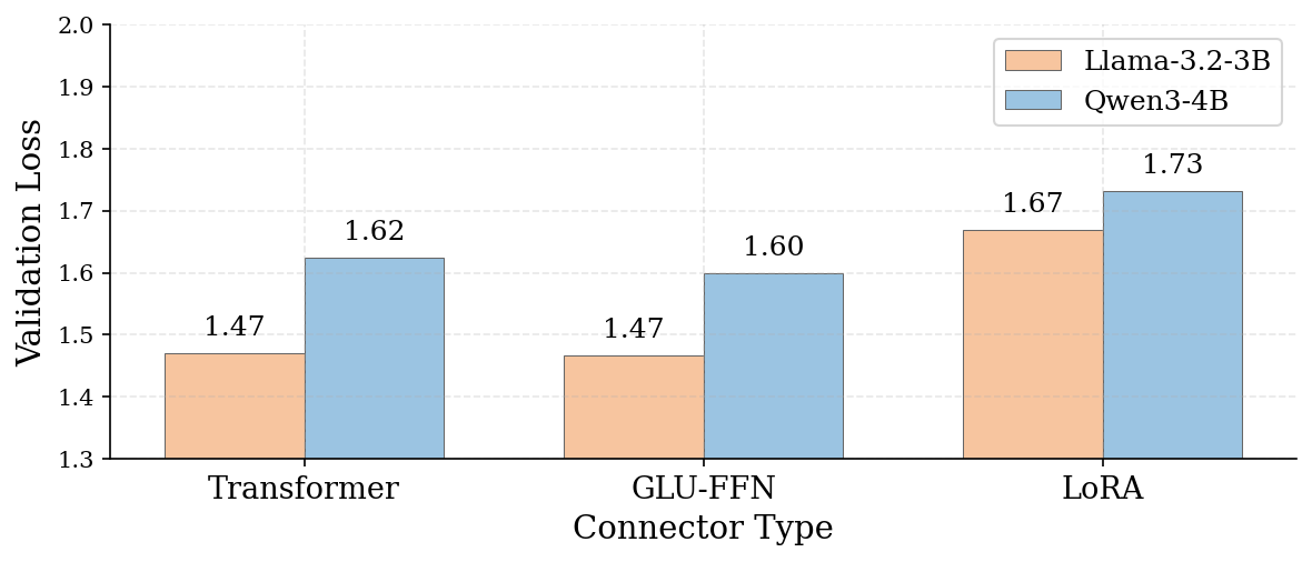
Table VIII confirms architecture-independent generalization, with Llama-3.2-3B consistently achieving lower loss than Qwen3-4B across all connector types. The ranking of Transformer > GLU-FFN > LoRA holds consistently for both models, suggesting the relative effectiveness of connector types is architecture-agnostic.

Notably, Llama-3.2-3B (3B parameters, 28 layers, $H$=3072) consistently outperforms larger Qwen3-4B (4B parameters, 36 layers, $H$=2560) by 0.12–0.13 loss for Transformer and GLU-FFN connectors. We observe two structural differences: (1) Llama has fewer layers to bridge (28 vs 36), and (2) Llama has a wider hidden dimension (3072 vs 2560). However, we cannot fully disentangle these factors from differences in pretraining data, tokenizer quality, and base model capabilities. The cross-architecture gap is somewhat larger for LoRA ($\Delta 0.16$ at $r=16$), suggesting that the architectural advantage extends to all connector types.

Table IX shows that Llama-3.2-3B achieves lower loss with fewer connector parameters across all connector types, quantifying the parameter efficiency advantage of shallower architectures. Llama-3.2-3B achieves 0.12 better loss than Qwen3-4B for Transformer connectors while using 23% fewer total connector parameters (82M vs 107M). The efficiency gap is even more pronounced when considering quality-per-parameter: Llama-3.2-3B achieves 1.47 loss with 82M parameters, while Qwen3-4B requires 107M parameters to achieve only 1.59 loss—wider and shallower architectures thus provide both better quality and lower memory requirements for skip-connector fine-tuning.

Communication Overhead Scaling

Table X reports data transfer volume, synchronization points, and bandwidth reduction for various connector configurations. Data volume per training step scales linearly with connector count and hidden dimension: for Qwen3-4B with gap-2 (17 connectors), each step transfers approximately 11.46 GB of activation and gradient data. Reducing to gap-15 (3 connectors) yields 82% bandwidth reduction, while the extreme gap-30 configuration achieves 94% reduction with only 0.67 GB/step. The key insight is that bandwidth reduction compounds with latency hiding. With gap-15, not only is data volume reduced by 82%, but the remaining transfers are hidden behind 15 layers of server computation. Combined with Top-K 5% gradient sparsification (additional 75% reduction), the effective bandwidth requirement drops from 11.46 GB/step to approximately 0.50 GB/step—a 23× total reduction that makes collaborative training practical over standard broadband connections.

The synchronization point count directly determines how many times the edge and server must wait for each other per training step. Fan-in placement reduces this to 1 regardless of connector count, which is particularly valuable for networks with high round-trip latency but adequate bandwidth. In contrast, uniform placement with gap-2 requires 13–17 synchronization points, making it unsuitable for high-latency scenarios despite potentially higher quality.

Ablation Studies

Skip connector performance depends on connector type, skip distance, and placement; we therefore conduct ablations to assess the generalizability of these design choices across architectures. Our results reveal consistent patterns: the connector ranking (Transformer > GLU-FFN > LoRA) and hyperparameter robustness are preserved for both Llama-3.2-3B and Qwen3-4B, suggesting that these findings generalize beyond our specific experimental configurations. Figure 6 illustrates successful and failed configurations.

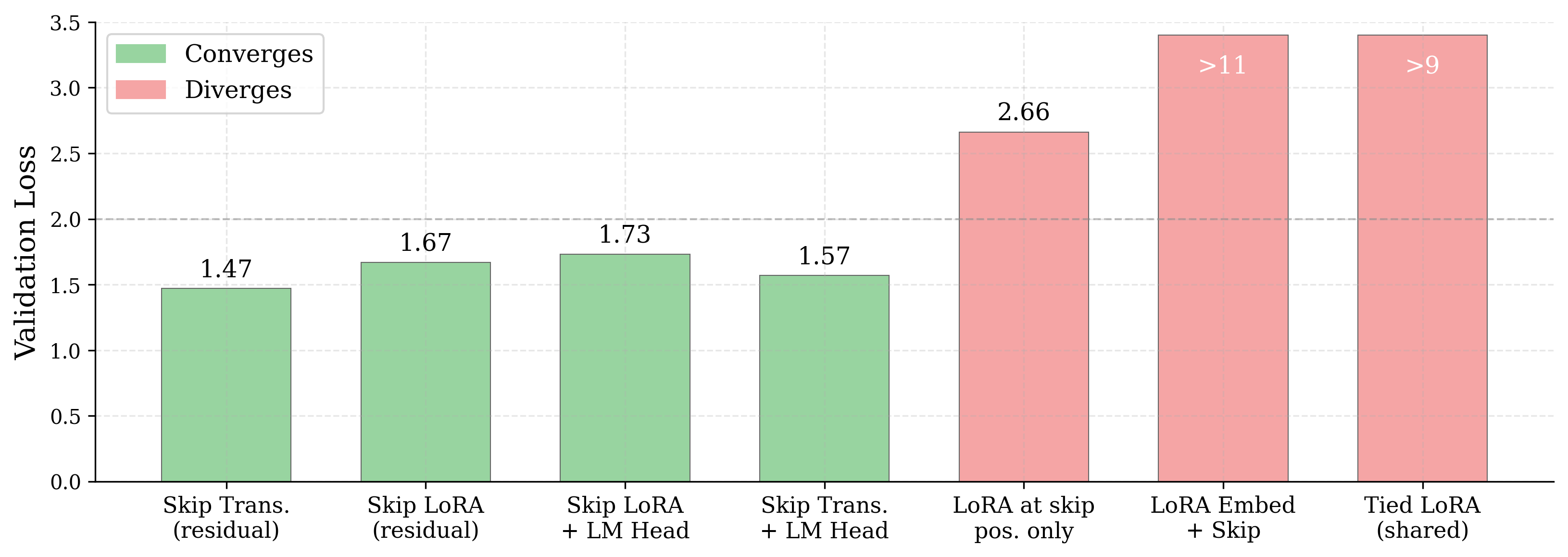
Skip residuals are essential. Removing the skip residual connection (Eq. 1) while keeping adapters at the same positions degrades performance from 1.73 to 2.66 loss ($\Delta$ = +0.93, 54% degradation). We tested this ablation at multiple skip distances (gap-2, gap-4, gap-15) with consistent results.

Embeddings cannot be approximated. To reduce edge-mode computational requirements, we evaluated replacing embedding matrices with SVD-initialized low-rank counterparts ($A = U_{:,:r} \sqrt{\Sigma_{:r}}$, $B = \sqrt{\Sigma_{:r}} V_{:r,:}^\top$). All configurations diverge to >11.0 loss across ranks 32–256, as embeddings encode token-level information in a fundamentally non-low-rank structure. For tied embedding-LM head models (Qwen3-4B), shared low-rank replacement fails catastrophically (>260 loss).

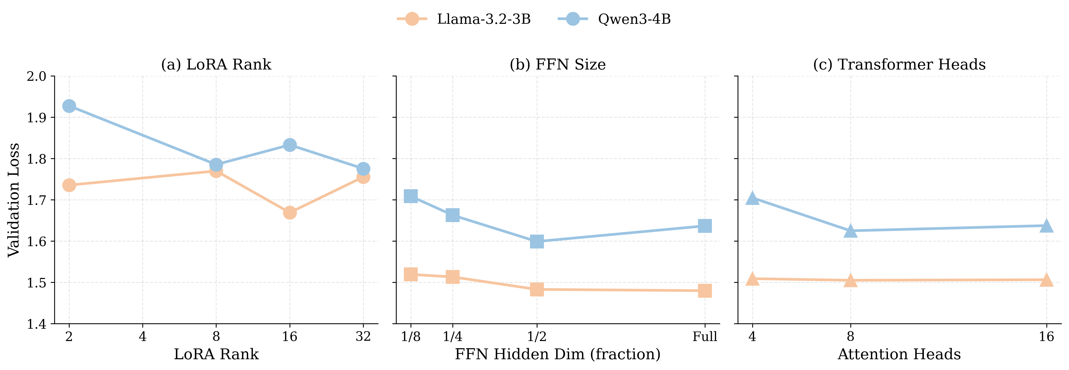
Hyperparameter robustness. Figure 7 demonstrates robustness across hyperparameter choices, with most configurations achieving results within $\pm 0.15$ loss on both architectures. For LoRA, ranks 2–32 yield similar performance on Llama-3.2-3B (with rank 16 best at 1.67), and on Qwen3-4B ranks 8/32 with longer training reach 1.78–1.79; the limited variation across ranks suggests the skip transformation is inherently low-rank. The architecture gap varies with rank: at ranks 8 and 32, the gap shrinks to only 0.02, suggesting that certain hyperparameter choices can partially compensate for architectural differences. For GLU-FFN, even 1/8 dimension achieves 1.52 loss on Llama-3.2-3B—only 0.04 worse than full dimension while using 8× fewer parameters per connector. On Qwen3, 1/4× matches 1/2× performance (1.60 loss), providing an 87.5% parameter reduction with minimal quality loss.

For Transformer connectors, 4–16 heads yield nearly identical results on Llama (0.01 variance) and similar results on Qwen3 (0.08 variance), indicating that the attention pattern learned for skip connections is simple enough that few heads suffice. Removing the FFN from Transformer connectors increases loss by only 0.12 (1.47→1.59 on Llama) while reducing parameters by approximately 40%. Overall, the robustness across all hyperparameter choices suggests that resource constraints can guide configuration selection without extensive tuning.

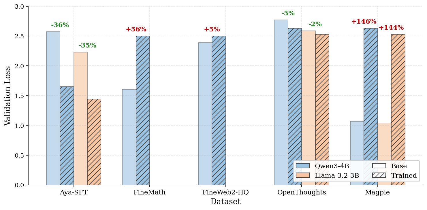
Figure 8 demonstrates that skip connectors generalize effectively to instruction-tuning tasks (Aya-SFT: 35–36% improvement) and reasoning tasks (OpenThoughts: 2–5%), which share long, coherent sequences. Training degrades performance on specialized text (FineMath: 56%, FineWeb2-HQ: 5%) and synthetic instruction-following (Magpie: 144–146%). For Magpie, the base model already achieves low loss (1.04–1.07), suggesting these synthetic examples closely match the pre-training distribution; skip connectors disrupt this alignment. The pattern suggests that skip connector effectiveness depends on how well the training data aligns with the model's pre-training distribution: highly aligned data (Magpie) sees degradation, while instruction-tuning and reasoning tasks benefit from the bridging mechanism.

Training Dynamics

Table XI compares final validation loss across training durations. Across all connector types and skip distances (gap-2, gap-15, gap-30 on Qwen3-4B), training converges smoothly within 10–15 optimizer steps; the frozen backbone (97.3% of parameters for Transformer) supplies stable gradients and zero-initialized residuals preserve pretrained behavior, yielding minimal validation-vs-training-loss gap. Most improvement is in the first 3 epochs (105 steps): Transformer/GLU-FFN gain <0.02 from extending to 10 epochs (350 steps) and nothing from 15 (555). LoRA gains more from longer training (0.07 from 105→350 on Llama) but also plateaus. More expressive connectors thus learn the skip transformation faster; short schedules (∼3 epochs) suffice for Transformer/GLU-FFN, ∼10 for LoRA.

VIDiscussion and Conclusion

BridgeLoRA represents a systems-optimized approach to model adaptation, prioritizing communication efficiency over expressivity by performing coherent corrections across multiple layers rather than localized per-layer modifications. BridgeLoRA addresses the three fundamental challenges.

Exposure Minimization

In Edge Fine-tuning Mode, the server processes only frozen-backbone activations; it never observes raw inputs, labels, loss values, or trainable-module parameters/gradients. This architectural separation keeps task-specific parameters and training signals on the edge. Cloud Offloading Mode trades some of this separation for efficiency by moving embeddings and loss computation to the server, but trainable connectors remain on the edge. The choice between modes depends on deployment requirements: Edge Fine-tuning Mode for stricter exposure control, Cloud Offloading Mode when fine-tuning must be more performant.

Privacy Properties

Federated-learning gradient-leakage attacks¹⁶ exploit gradients of trainable parameters w.r.t. a labeled batch. In BridgeLoRA the only gradients crossing the boundary are w.r.t. frozen backbone activations; connector parameter gradients $\nabla_{\theta_C}\mathcal{L}$ stay on the edge in both modes, and Edge Fine-tuning Mode additionally hides labels and the loss. Activations remain a leakage surface as in split learning^18,19, but BridgeLoRA reduces this surface to $L/d$ states; combining with differential privacy¹⁷ is a natural complement.

Lightweight Edge Computation

Skip connectors enable edge devices to participate in fine-tuning by limiting their role to lightweight computation. The edge trains only 2.7% of parameters (for Transformer connectors on Llama) while the server handles all frozen-backbone forward and backward passes. On Aya-SFT, Transformer skip connectors outperform standard LoRA on the same model (1.47 vs. 1.66 validation loss on Llama-3.2-3B). The frozen backbone acts as an implicit regularizer: training and validation curves track closely, and convergence happens within 3 epochs. Connector expressiveness matters: the ranking Transformer > GLU-FFN > LoRA holds consistently, with more expressive connectors better capturing the transformation needed to bridge skipped layers. Llama-3.2-3B (28 layers) outperforms the larger Qwen3-4B (36 layers) by $\Delta 0.12$; while we cannot fully disentangle contributing factors, this pattern is consistent with bridging difficulty scaling with depth rather than capacity.

Communication Efficiency

Skip distance directly controls the quality-communication trade-off. Gap-15 reduces round-trips by 85% (from 13 to 2 connectors on Llama) with only 0.10–0.12 loss degradation for Transformer and GLU-FFN connectors; a single connector bridging 30 layers achieves 1.82 loss, remaining competitive with standard LoRA. Our distributed testbed experiments show that 500ms added latency increases step time by 44%, yet validation loss remains unchanged, confirming that reduced synchronization frequency effectively mitigates latency impact. Bandwidth can be reduced aggressively: Top-K sparsification at 5% achieves 75% compression with only 0.3% quality degradation, and combining INT8 with Top-K 1% yields 40× compression with 0.9% quality degradation. Inference uses the same $L/d$ synchronization points as one training forward pass, so a configuration tuned for training (e.g., gap-15) should be the relevant operating point for serving; end-to-end inference benchmarks are future work.

Configuration Guidance

Hyperparameter ablations are flat within $\pm 0.15$ loss across LoRA rank 2–32, FFN width 1/8–full, and Transformer heads 4–16, so configuration can be chosen by deployment constraint rather than by search. Default recipe: Transformer at gap-2; if bandwidth/latency-constrained, increase to gap-15 or use fan-in placement ($\mathcal{O}(1)$ sync points); if parameter/memory-constrained, drop to GLU-FFN at 1/4×, falling back to LoRA only when GLU-FFN is unaffordable.

Our results reveal a fundamental tension between exposure minimization and practicality. Edge Fine-tuning Mode provides maximum separation, but at 89s/step (at 20ms latency) the training time is substantial. Cloud Offloading Mode achieves 56s/step (1.6× faster) by transmitting only connector activations/gradients rather than the full backbone round-trips that Edge Mode requires, but at the cost of trusting the server with labels and loss. In practice, Cloud Offloading Mode represents the viable path for fine-tuning tasks that require the trained parameters to reside on the edge devices. The observation that shallower models outperform deeper ones suggests that width should be prioritized over depth in architectures intended for skip bridging.

Limitations

Several evaluation axes remain open. (i) Validation loss is standard for parameter-efficient fine-tuning^1,2 but does not directly capture downstream task accuracy; benchmark-style evaluation is future work. (ii) Our testbed uses supercomputer nodes with simulated WAN latency; real cellular/satellite edge devices and federated-learning baselines are immediate next steps. (iii) Sequences are $\leq 512$ tokens and training runs to 555/350 steps on Llama/Qwen3; longer contexts and schedules remain unexplored. (iv) BridgeLoRA provides exposure minimization, not cryptographic privacy; intermediate activations may leak via inversion¹⁹, and we provide neither empirical leakage analysis nor a formal bound (DP is a natural complement). (v) The protocol assumes stable connections and does not address fault tolerance.

These results establish skip connectors as a principled approach to exposure-minimizing collaborative fine-tuning, enabling adaptation of billion-parameter models on edge devices while keeping task-specific parameters local.